Incorporating Geospatial Context into Risk Modelling

Overview

This project demonstrates how geospatial context can be incorporated into predictive risk models using aggregated, non‑identifying spatial features. The emphasis is on feature construction, spatial smoothing, and avoiding information leakage rather than on fine‑grained location data.

All data used in this project is synthetic or publicly available.

---

Problem Statement

We consider a hypothetical risk prediction problem where event likelihood varies spatially due to underlying environmental, behavioural, or socio‑economic factors. The goal is to construct geospatial features that capture this variation in a stable and privacy‑preserving way.

Key challenges include:

• Spatial leakage
• Sparsity in fine‑grained locations
• Balancing resolution with robustness

---

Synthetic Spatial Data

import numpy as np
import pandas as pd

np.random.seed(123)

n = 20000

# Synthetic latitude / longitude (approximate UK bounding box)
lat = np.random.uniform(50.0, 55.5, n)
lon = np.random.uniform(-5.5, 1.8, n)

df = pd.DataFrame({
    "latitude": lat,
    "longitude": lon
})

df.head()

	latitude	longitude
0	53.830581	-4.868714
1	51.573766	-1.235600
2	51.247683	-2.048911
3	53.032231	-0.370855
4	53.957079	-2.130276

---

Create spatial clusters of higher risk

risk_centers = [
    (51.5, -0.1),   # London
    (53.5, -2.3),   # Manchester
    (52.5, -1.9)    # Birmingham
]

risk = np.zeros(n)

for lat_c, lon_c in risk_centers:
    dist = np.sqrt((df["latitude"] - lat_c)**2 + (df["longitude"] - lon_c)**2)
    risk += np.exp(-dist / 0.5)

# Normalise
risk = risk / risk.max()

df["spatial_risk"] = risk

df.head()

	latitude	longitude	spatial_risk
0	53.830581	-4.868714	0.006423
1	51.573766	-1.235600	0.195246
2	51.247683	-2.048911	0.099452
3	53.032231	-0.370855	0.092219
4	53.957079	-2.130276	0.387473

---

Event Generation

logit = -4.0 + 2.0 * df["spatial_risk"]
prob = 1 / (1 + np.exp(-logit))

df["event"] = np.random.binomial(1, prob)

df["event"].mean()

np.float64(0.02315)

---

Spatial Binning

To incorporate spatial context in a robust and privacy‑preserving way, we discretise latitude and longitude into coarse spatial bins. This reduces sensitivity to exact coordinates while enabling aggregation of local risk signals.

# Define bin sizes (degrees)
lat_bin_size = 0.25
lon_bin_size = 0.25

df["lat_bin"] = (df["latitude"] / lat_bin_size).astype(int)
df["lon_bin"] = (df["longitude"] / lon_bin_size).astype(int)

# Combine into a single spatial cell identifier
df["spatial_cell"] = df["lat_bin"].astype(str) + "_" + df["lon_bin"].astype(str)

df[["latitude", "longitude", "spatial_cell"]].head()

	latitude	longitude	spatial_cell
0	53.830581	-4.868714	215_-19
1	51.573766	-1.235600	206_-4
2	51.247683	-2.048911	204_-8
3	53.032231	-0.370855	212_-1
4	53.957079	-2.130276	215_-8

---

Spatial Aggregation

Within each spatial cell, we compute aggregated statistics that summarise local event behaviour. These aggregates form the basis of geospatial risk features.

cell_stats = (
    df.groupby("spatial_cell")
      .agg(
          cell_event_rate=("event", "mean"),
          cell_event_count=("event", "sum"),
          cell_exposure=("event", "count")
      )
      .reset_index()
)

cell_stats.head()

	spatial_cell	cell_event_rate	cell_event_count	cell_exposure
0	200_-1	0.030303	1	33
1	200_-10	0.000000	0	39
2	200_-11	0.041667	1	24
3	200_-12	0.000000	0	39
4	200_-13	0.055556	2	36

---

Smoothing Sparse Spatial Estimates

Raw cell event rates can be noisy when exposure is low.
We’ll apply empirical Bayes–style smoothing.

To reduce variance in low‑exposure cells, we apply simple Bayesian smoothing by shrinking cell‑level event rates toward the global mean.

# Global event rate
global_rate = df["event"].mean()

# Smoothing strength (pseudo-counts)
alpha = 50

cell_stats["smoothed_event_rate"] = (
    (cell_stats["cell_event_rate"] * cell_stats["cell_exposure"] + alpha * global_rate)
    / (cell_stats["cell_exposure"] + alpha)
)

cell_stats.head()

	spatial_cell	cell_event_rate	cell_event_count	cell_exposure	smoothed_event_rate
0	200_-1	0.030303	1	33	0.025994
1	200_-10	0.000000	0	39	0.013006
2	200_-11	0.041667	1	24	0.029155
3	200_-12	0.000000	0	39	0.013006
4	200_-13	0.055556	2	36	0.036715

---

Constructing Geospatial Features

We attach the aggregated spatial features back to the individual‑level dataset for use in downstream modelling.

df = df.merge(
    cell_stats[["spatial_cell", "smoothed_event_rate"]],
    on="spatial_cell",
    how="left"
)

df[["latitude", "longitude", "smoothed_event_rate"]].head()

	latitude	longitude	smoothed_event_rate
0	53.830581	-4.868714	0.014652
1	51.573766	-1.235600	0.027660
2	51.247683	-2.048911	0.041006
3	53.032231	-0.370855	0.028019
4	53.957079	-2.130276	0.028388

---

from shapely.geometry import Point
import geopandas as gpd

geometry = [
    Point(lon, lat)
    for lon, lat in zip(df["longitude"], df["latitude"])
]

gdf = gpd.GeoDataFrame(df, geometry=geometry, crs="EPSG:4326")
gdf_bng = gdf.to_crs(epsg=27700)

---

Visualising Raw Spatial Events

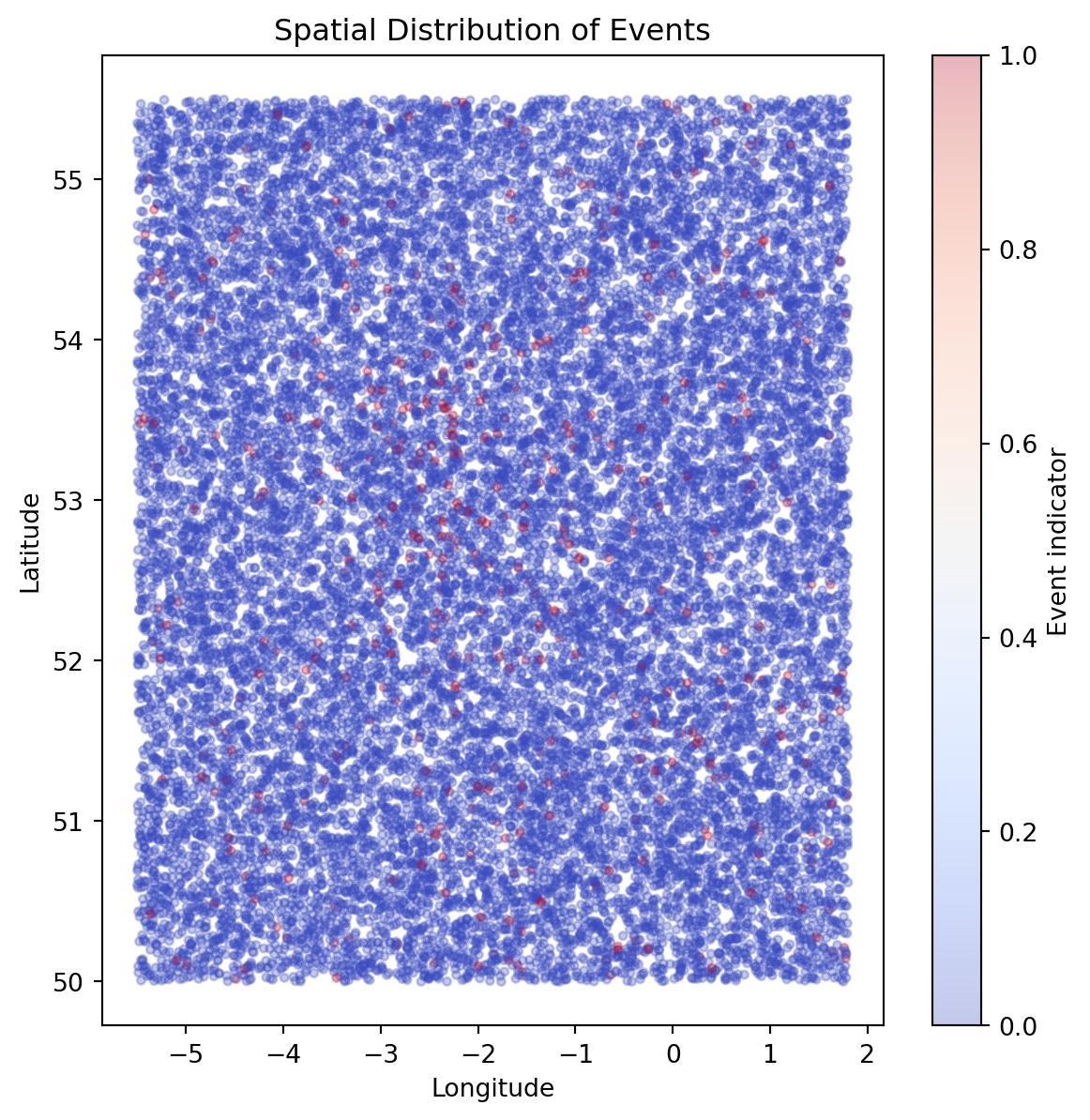
We begin by visualising the spatial distribution of events to understand broad geographic patterns and clustering behaviour.

import matplotlib.pyplot as plt

plt.figure(figsize=(7, 7))

plt.scatter(
    df["longitude"],
    df["latitude"],
    c=df["event"],
    cmap="coolwarm",
    alpha=0.3,
    s=10
)

plt.xlabel("Longitude")
plt.ylabel("Latitude")
plt.title("Spatial Distribution of Events")
plt.colorbar(label="Event indicator")
plt.show()

---

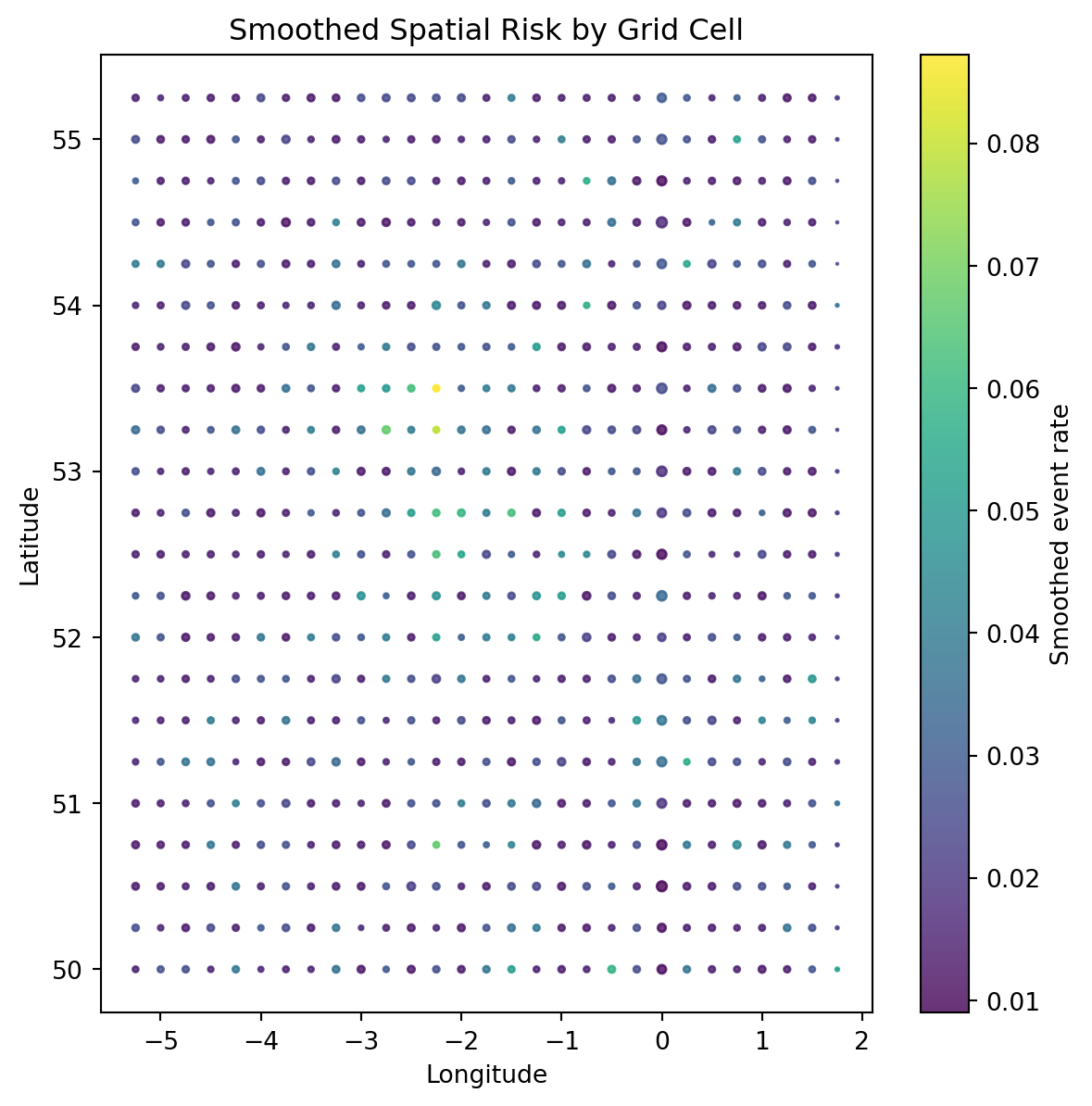
Visualising Smoothed Spatial Risk

Aggregated and smoothed spatial features provide a clearer view of underlying geographic risk patterns.

# Use cell-level centroids for plotting
cell_stats["lat_center"] = (
    cell_stats["spatial_cell"]
    .str.split("_")
    .str[0]
    .astype(int) * lat_bin_size
)

cell_stats["lon_center"] = (
    cell_stats["spatial_cell"]
    .str.split("_")
    .str[1]
    .astype(int) * lon_bin_size
)

plt.figure(figsize=(7, 7))

plt.scatter(
    cell_stats["lon_center"],
    cell_stats["lat_center"],
    c=cell_stats["smoothed_event_rate"],
    cmap="viridis",
    s=cell_stats["cell_exposure"] / 5,
    alpha=0.8
)

plt.xlabel("Longitude")
plt.ylabel("Latitude")
plt.title("Smoothed Spatial Risk by Grid Cell")
plt.colorbar(label="Smoothed event rate")
plt.show()

Comparing individual‑level and aggregated spatial visualisations highlights the trade‑off between noise and signal. While raw location data is highly variable, spatial aggregation and smoothing reveal stable geographic patterns suitable for use in predictive models.

---

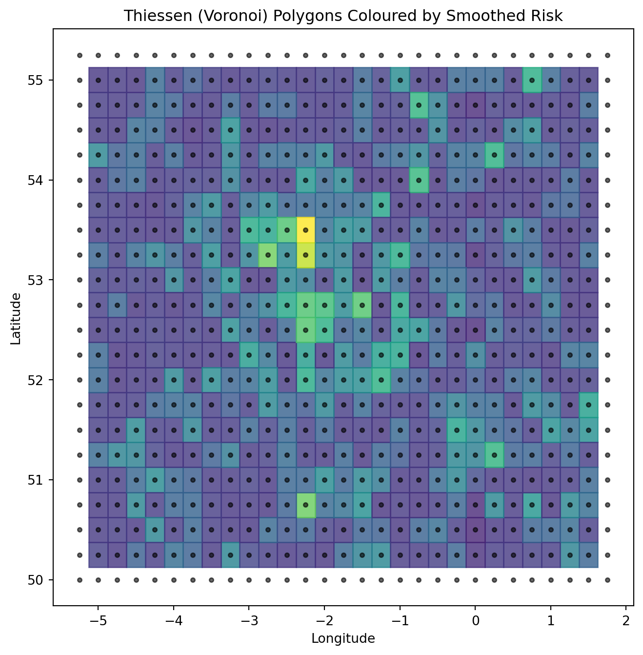
Thiessen (Voronoi) Polygons for Spatial Risk

To further visualise spatial structure, we construct Thiessen (Voronoi) polygons based on spatial cell centroids. Each polygon represents the region of space closest to a given cell, providing a continuous spatial partition coloured by smoothed risk.

For the curious, click here to learn more about Voronoi polygons

import numpy as np
import matplotlib.pyplot as plt
from scipy.spatial import Voronoi

# Prepare centroid coordinates
points = np.column_stack([
    cell_stats["lon_center"].values,
    cell_stats["lat_center"].values
])

# Compute Voronoi tessellation
vor = Voronoi(points)

# Plot
plt.figure(figsize=(8, 8))

# Plot Voronoi regions
for region_index, region in enumerate(vor.regions):
    if not region or -1 in region:
        continue  # Skip infinite regions

    polygon = [vor.vertices[i] for i in region]
    polygon = np.array(polygon)

    # Find corresponding point index
    point_indices = np.where(vor.point_region == region_index)[0]
    if len(point_indices) == 0:
        continue

    idx = point_indices[0]
    risk_value = cell_stats.iloc[idx]["smoothed_event_rate"]

    plt.fill(
        polygon[:, 0],
        polygon[:, 1],
        color=plt.cm.viridis(risk_value / cell_stats["smoothed_event_rate"].max()),
        alpha=0.8
    )

# Overlay centroids
plt.scatter(
    cell_stats["lon_center"],
    cell_stats["lat_center"],
    c="black",
    s=10,
    alpha=0.6
)

plt.xlabel("Longitude")
plt.ylabel("Latitude")
plt.title("Thiessen (Voronoi) Polygons Coloured by Smoothed Risk")
plt.show()

---

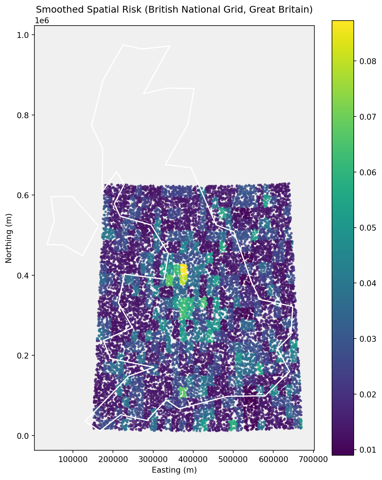
Mapping Spatial Risk Using the British National Grid

To visualise spatial risk in a cartographically appropriate coordinate system, we project locations onto the British National Grid (BNG). This projection is commonly used for mapping and spatial analysis within Great Britain, providing distance‑preserving coordinates in metres.

Northern Ireland uses a separate national grid and is therefore excluded from this visualisation for technical correctness.

import geopandas as gpd
from shapely.geometry import Point

# Load Natural Earth country boundaries (110m resolution)
url = "https://naturalearth.s3.amazonaws.com/110m_cultural/ne_110m_admin_0_countries.zip"

world = gpd.read_file(url)

# Extract United Kingdom
uk = world[world["NAME"] == "United Kingdom"]

uk

	featurecla	scalerank	LABELRANK	SOVEREIGNT	SOV_A3	ADM0_DIF	LEVEL	TYPE	TLC	ADMIN	...	FCLASS_TR	FCLASS_ID	FCLASS_PL	FCLASS_GR	FCLASS_IT	FCLASS_NL	FCLASS_SE	FCLASS_BD	FCLASS_UA	geometry
143	Admin-0 country	1	2	United Kingdom	GB1	1	2	Country	1	United Kingdom	...	None	None	None	None	None	None	None	None	None	MULTIPOLYGON (((-6.19788 53.86757, -6.95373 54...

1 rows × 169 columns

---

# Convert point data to GeoDataFrame
geometry = [
    Point(lon, lat)
    for lon, lat in zip(df["longitude"], df["latitude"])
]

gdf = gpd.GeoDataFrame(df, geometry=geometry, crs="EPSG:4326")

# Reproject to British National Grid (EPSG:27700)
uk_bng = uk.to_crs(epsg=27700)

uk_bng

	featurecla	scalerank	LABELRANK	SOVEREIGNT	SOV_A3	ADM0_DIF	LEVEL	TYPE	TLC	ADMIN	...	FCLASS_TR	FCLASS_ID	FCLASS_PL	FCLASS_GR	FCLASS_IT	FCLASS_NL	FCLASS_SE	FCLASS_BD	FCLASS_UA	geometry
143	Admin-0 country	1	2	United Kingdom	GB1	1	2	Country	1	United Kingdom	...	None	None	None	None	None	None	None	None	None	MULTIPOLYGON (((124122.565 449434, 76073.084 4...

1 rows × 169 columns

Keep only Great Britain (approximate longitude filter)

uk_gb = uk[uk.geometry.centroid.x > -8]

uk_gb_bng = uk_gb.to_crs(epsg=27700)

C:\Users\morri\AppData\Local\Temp\ipykernel_38060\2014797042.py:1: UserWarning:

Geometry is in a geographic CRS. Results from 'centroid' are likely incorrect. Use 'GeoSeries.to_crs()' to re-project geometries to a projected CRS before this operation.

---

from shapely.geometry import Point
import geopandas as gpd

geometry = [
    Point(lon, lat)
    for lon, lat in zip(df["longitude"], df["latitude"])
]

gdf = gpd.GeoDataFrame(df, geometry=geometry, crs="EPSG:4326")
gdf_bng = gdf.to_crs(epsg=27700)

gdf_bng.head()

	latitude	longitude	spatial_risk	event	lat_bin	lon_bin	spatial_cell	smoothed_event_rate	geometry
0	53.830581	-4.868714	0.006423	0	215	-19	215_-19	0.014652	POINT (211310.296 440963.865)
1	51.573766	-1.235600	0.195246	0	206	-4	206_-4	0.027660	POINT (453071.279 186376.537)
2	51.247683	-2.048911	0.099452	0	204	-8	204_-8	0.041006	POINT (396682.661 149835.711)
3	53.032231	-0.370855	0.092219	0	212	-1	212_-1	0.028019	POINT (509347.525 349568.357)
4	53.957079	-2.130276	0.387473	0	215	-8	215_-8	0.028388	POINT (391549.07 451228.895)

---

import matplotlib.pyplot as plt

fig, ax = plt.subplots(figsize=(8, 10))

# Set subtle background colour
ax.set_facecolor("#f0f0f0")

# Plot spatial risk points first
gdf_bng.plot(
    ax=ax,
    column="smoothed_event_rate",
    cmap="viridis",
    markersize=5,
    alpha=0.7,
    legend=True
)

# Plot GB boundary ON TOP as white outline
uk_gb_bng.plot(
    ax=ax,
    facecolor="none",
    edgecolor="white",
    linewidth=1.5
)

ax.set_title("Smoothed Spatial Risk (British National Grid, Great Britain)")
ax.set_xlabel("Easting (m)")
ax.set_ylabel("Northing (m)")

plt.show()

---

Country boundaries are sourced from Natural Earth (public domain) and projected into the British National Grid (EPSG:27700). Northern Ireland is excluded due to its use of a separate national grid reference system.

---

WIP - Visualisation

---

import geopandas as gpd

lsoa = gpd.read_file(r"C:\Users\morri\PycharmProjects\shmers.github.io\geodata\Lower_layer_Super_Output_Areas_December_2021_Boundaries_EW_BGC_V5_-6970154227154374572.gpkg")

lsoa.head()

	LSOA21CD	LSOA21NM	LSOA21NMW	BNG_E	BNG_N	LAT	LONG	GlobalID	geometry
0	E01000001	City of London 001A		532123	181632	51.518169	-0.097150	{86214465-5CF4-4E8F-9492-3667471C42D6}	MULTIPOLYGON (((532105.312 182010.574, 532104....
1	E01000002	City of London 001B		532480	181715	51.518829	-0.091970	{CD40C491-6567-405F-8C18-426E17B356CE}	MULTIPOLYGON (((532634.497 181926.016, 532572....
2	E01000003	City of London 001C		532239	182033	51.521740	-0.095330	{7FD27AAF-D858-4E46-9099-92B43F66B948}	MULTIPOLYGON (((532135.138 182198.131, 532071....
3	E01000005	City of London 001E		533581	181283	51.514690	-0.076280	{7E76A16A-028F-4F49-84B5-6E5A67322F3C}	MULTIPOLYGON (((533808.018 180767.774, 533842....
4	E01000006	Barking and Dagenham 016A		544994	184274	51.538750	0.089317	{25AB047E-6FCF-4F76-9176-E92E44C0E097}	MULTIPOLYGON (((545122.049 184314.931, 545118....

---

Reproject to BNG

lsoa_bng = lsoa.to_crs(epsg=27700)

lsoa_bng.crs

<Projected CRS: EPSG:27700>
Name: OSGB36 / British National Grid
Axis Info [cartesian]:
- E[east]: Easting (metre)
- N[north]: Northing (metre)
Area of Use:
- name: United Kingdom (UK) - offshore to boundary of UKCS within 49°45'N to 61°N and 9°W to 2°E; onshore Great Britain (England, Wales and Scotland). Isle of Man onshore.
- bounds: (-9.01, 49.75, 2.01, 61.01)
Coordinate Operation:
- name: British National Grid
- method: Transverse Mercator
Datum: Ordnance Survey of Great Britain 1936
- Ellipsoid: Airy 1830
- Prime Meridian: Greenwich

---

LSOA boundary data are sourced from the UK Office for National Statistics Open Geography Portal and stored locally to ensure reproducibility. This avoids reliance on unstable external URLs while preserving authoritative geography under the Open Government Licence.

---

Load population CSV

pop = pd.read_csv(r"C:\Users\morri\PycharmProjects\shmers.github.io\geodata\Mid 2022 LSOA 2021.csv")
print(pop.columns.tolist())

pop.head()

['LAD 2023 Code', 'LAD 2023 Name', 'LSOA 2021 Code', 'LSOA 2021 Name', 'Total', 'F0 to 15', 'F16 to 29', 'F30 to 44', 'F45 to 64', 'F65 and over', 'M0 to 15', 'M16 to 29', 'M30 to 44', 'M45 to 64', 'M65 and over']

	LAD 2023 Code	LAD 2023 Name	LSOA 2021 Code	LSOA 2021 Name	Total	F0 to 15	F16 to 29	F30 to 44	F45 to 64	F65 and over	M0 to 15	M16 to 29	M30 to 44	M45 to 64	M65 and over
0	E06000001	Hartlepool	E01011949	Hartlepool 009A	1,876	182	166	189	274	179	189	181	152	236	128
1	E06000001	Hartlepool	E01011950	Hartlepool 008A	1,117	96	79	102	147	99	104	92	138	175	85
2	E06000001	Hartlepool	E01011951	Hartlepool 007A	1,260	90	126	139	170	90	133	100	146	189	77
3	E06000001	Hartlepool	E01011952	Hartlepool 002A	1,635	193	134	156	207	196	194	109	104	202	140
4	E06000001	Hartlepool	E01011953	Hartlepool 002B	1,984	216	220	190	231	145	290	177	160	232	123

---

Extract relevant columns

pop = pop.rename(columns={
    "LSOA 2021 Code": "LSOA21CD",
    "Total": "population"
})

pop = pop[["LSOA21CD", "population"]]

pop.head()

	LSOA21CD	population
0	E01011949	1,876
1	E01011950	1,117
2	E01011951	1,260
3	E01011952	1,635
4	E01011953	1,984

pop["population"] = (
    pop["population"]
    .str.replace(",", "", regex=False)
    .astype(int)
)

pop.dtypes

LSOA21CD      object
population     int64
dtype: object

lsoa = lsoa.merge(
    pop,
    on="LSOA21CD",
    how="left"
)

lsoa["population"].isna().mean()

np.float64(0.0)

---

## Project & Compute Population Density

lsoa_bng = lsoa.to_crs(epsg=27700)

lsoa_bng["area_km2"] = lsoa_bng.geometry.area / 1e6
lsoa_bng["pop_density"] = (
    lsoa_bng["population"] / lsoa_bng["area_km2"]
)

import matplotlib.pyplot as plt

fig, ax = plt.subplots(figsize=(9, 11))
ax.set_facecolor("#f0f0f0")

lsoa_bng.plot(
    ax=ax,
    column="pop_density",
    cmap="viridis",
    linewidth=0,
    legend=True,
    legend_kwds={
        "label": "Population density (people per km²)",
        "shrink": 0.6
    }
)

ax.set_title("Population Density by LSOA (Great Britain)")
ax.set_axis_off()
plt.show()